HKSFC Licensed Corp #ADC118
FIXED INCOME INVESTMENTS

Zihaiquo 自嗨锅 completed more than RMB 100 million of Round B financing
May 15, 2020
2020 1H Global Asset Allocation Portfolio Review
July 9, 2020FIXED INCOME INVESTMENTS
Learning outcomes
Upon completion of this chapter, learners should be able to:
- Describe the characteristics of different types of bond, including straight or “plain vanilla” bond, zero coupon bond, callable and puttable bond, convertible bond and other types of bond
- Understand the relationships between a bond’s price, coupon rate, maturity and market discount rate
- Calculate a bond’s price given a market discount rate
- Explain and calculate the clean price, accrued interest and dirty price of a bond
- Identify the relationship between interest rate expectation and yield curve
- Describe the various risks of investing in bonds.
Introduction
Fixed income instruments are one of the examples of money market instruments. Pricing models and various terms, and interactions between bond prices and interest rates are introduced in this chapter, providing the background for learners to understand the sensitivity of fixed income instruments.
Besides this, different risks arising from investing in bonds are covered because the risks influence bond prices significantly. Learners have to understand the differences between the rsks and develop their knowledge of risk management.
Term Structure of Interest Rate
The relationship between the yields on comparable risk bonds with different maturities (short to long-term) is called the term structure of interest rates. The graph that depicts this relationship is the yield curve.
The yield curve is usually constructed with highly-rated government-issued debt securities, which are commonly used as a benchmark for setting yields in many other sectors of the debt market. The yield curve is also a tool to allow market participants to forecast the future direction of interest rates and inflation in an economy.
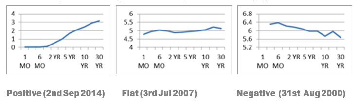
There are three possible shapes to a yield curve.
Upward-sloping
This is the normal situation in which yields increase with the term to maturity. As there is greater risk in tying up money longer for longer term bonds, investors demand higher yields in compensation. Therefore a positive relationship between yield and maturity shows up in the yield curve. An upward-sloping yield curve is consistent with an expectation of interest rates rising in the future. Therefore it is associated with expectation of economic expansion and rising inflation.
Downward-sloping
A downward-sloping yield curve depicts a general decline in yields, as maturity increases. Since long-term interest rates are lower than short-term ones, a negative yield curve is associated with an expectation of falling interest rates, economic recession and even deflation.
Flat
A flat yield curve reflects market expectations of stable interest rates. A flat yield curve may indicate a period of transition between positive and negative yield.
![]()
![]()
![]()
U.S. Treasury Yield Curve (X-Axis: Maturity; Y-Axis: Yield (%))
The yield spread is the difference between yields on different bonds, particularly with
government bonds. It allows for comparisons of yields of two different products. There are three different ways to calculate a yield spread.
One way is to deduct the yield of one instrument from the other one, an approach known as “absolute yield spread.”
A second way, known as “relative yield spread”, uses the difference in the yield between bonds measured in basis points. Thus the yield on a bond, subtracting the yield on the other bond and dividing by the yield of that bond produces the relative yield spread.
And finally there is the yield ratio, which measures the ratio of yield between bonds, by dividing the yield on a bond by the yield of another bond.
It has been found that lower quality issuers with larger yield spread with government bonds and longer-term bonds usually face more interest rate volatility, that is percentage change in bond price is higher, when market yield changes.
Bond pricing and yield
The following sections illustrate some fundamental concepts that are crucial to a basic understanding of bond pricing and yield.
Time value of money
The concept of the time value of money refers to the relationship between present and fiiture values of money. A dollar that can be invested now is worth more to an investor than a dollar that will be invested at some time in the future, because money that is invested now will be worth more to the investor in the future, with the effect of interest income. The same amount of money that will become available to an investor at some time in the future, if considered in terms of its current value (with the interest component), is worth less now.
For example, a dollar invested today will return, at a specific future date, both the original dollar and some interest. Assume you invest HKD100 for one year at 10%. At the end of the year, your return would be HKD110 (100 plus 10 interest). In this example, the time value of money is 10%. The time value or interest rate is the reward for the investor.
HKD100 x (1 + 10%) = HKD110
The HKD100 the investor has today is called present value, while the HKD110 he will receive in the future is called the future value (of the original HKD100).
Quoting interest rates
Nominal interest rates: the most common way of quoting annual interest rates, without considering the compounding effect.
Rea1 interest rates: take into account changes in the purchasing power of money over time, i.e. inflation. The relationships concerned with nominal interest rate, real interest rate and inflation are:
(1 + nominal interest rate) = (1 + real interest rate) ^ (1 + inflation rate).
Effective interest rates: annual interest rates quoted with different compounding periods that cannot be compared directly. The effective interest rate takes account of different compounding periods in nominal rates and adjusts the rates to a common basis (usually annual) for comparative purposes.
For example, assume you wish to invest HKD100 for one year and you are offered the following annual interest rates:
- 7.50% paid monthly
- 7.75% paid quarterly
- 8% paid semi-annually
Which offers the highest return?
To compare these nominal interest rates, we need to convert them to effective interest rates, using the formula:
EAR = (1+ R/n)^n – 1
where
EAR = Effective Interest Rate
R = Nominal Interest Rate
n = no. of interest payment
7.50% paid monthly:
EAR = (7.50% / 12) ^ 12 = 7.95%
7.75% paid quarterly:
EAR = (7.75% / 4) ^ 4 = 7.76%
8.00% paid semi-annually:
EAR = (8% / 2) ^ 2 = 8.16%
In this example, the 8.00% interest rate paid semi-annually gives the highest return.
It should be noted that in some jurisdictions, especially in relation to credit-card interest rates and loans, effective interest rates must be the ones publicized (not nominal rates).
Price yield relationship
The bond price moves inversely with the market interest rate. If the interest rate rises, the bond price falls; if the interest rate falls, the bond price increases. This relationship can be confirmed through the bond valuation formula depicted in section 3.5.1 below. With an increase in the interest rate, the present value of future cash flows will be smaller and hence the bond price is lower. The diagram below shows the price-yield profile, also called the price-yield curve. Notice that the curve is convex. This is known as positive convexity as bond prices go up faster than they go down. In other words, a 1% decrease in interest rate has a greater impact on the bond price than a 1% increase.
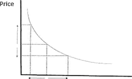
Yield
Diagram 4: Price-yield relationship of a bond
A bond with a relatively high yield indicates that it is perceived by investors as being a risky investment. Therefore its value, or price, is lower. Conversely, a bond with a relatively low yield indicates that investors perceive it as a low-risk investment. Therefore, its value, or price, is higher.
When the current market interest rate falls below the coupon rate, the bond price is always higher than the par value, i.e. the bond is traded at a premium. When the current market interest rate is equal to the coupon rate, the bond price is the same as the par value, i.e. the bond trades at par. When the current market interest rate rises above the coupon rate, the bond price is always lower than the par value, i.e. the bond is traded at a discount.
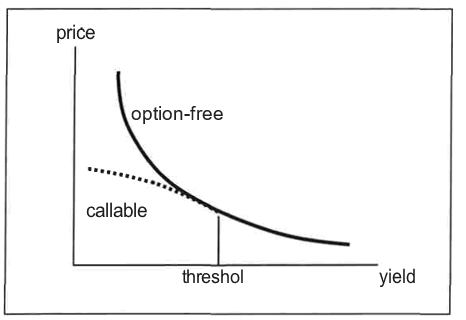
Diagram 5: Price-yield curves of option-free and callable bonds
In the case of a callable bond, when the interest rate falls below a certain threshold, the price-yield relationship becomes concave, i.e. it exhibits negative convexity. This arises from price compression as the bond price approaches the call price, which acts as a cap on the bond’s value. In this case, a 1% increase in the interest rate has a larger impact on the bond price than a 1% decrease in the rate. In other words, negative convexity limits the price performance of a callable bond when interest rates fall.
Price convergence and maturity
Suppose that the market interest rate remains the same from the time the bond is bought and the maturity date. What will happen to the bond price? For a bond sold at par, the price will remain at par as it approaches the maturity date. If a bond is sold at a premium, its price will decrease gradually as it approaches the maturity date. On the maturity date and after receiving the last coupon, the bond price is equal to the par value. If a bond is sold at a discount, its price will increase gradually as it moves towards the maturity date. On the maturity date and after receiving the last coupon, the bond price is equal to the par value. The diagram below shows the relationship between maturity and price convergence when the interest rate remains constant.
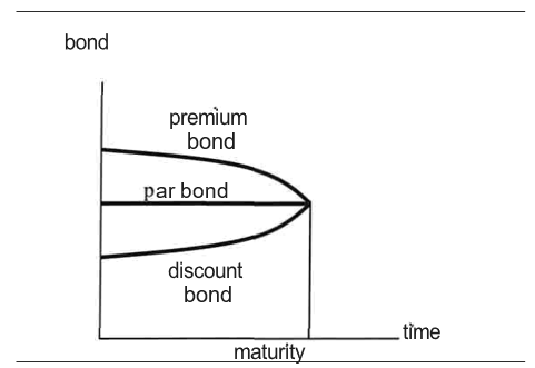
Diagram 6: Price convergence and maturity
Bond price volatility
The future cash flows of a bond have two components: periodic coupons and the more substantial par value at maturity. If the maturity period increases, the par value portion of future cash flows will be discounted over a longer period. The change in the present value of the bond due to the par value is more than outweighed by the change in the present value in the opposite direction due to an increase in the total number of coupons. Hence, for a given change in market interest rates, bonds with a longer maturity will show more price volatility than those with a shorter maturity. However, the effect of extending the maturity of a bond has a proportionately smaller effect on bond price volatility because of the nature of discounting. In other words, price volatility increases at a diminishing rate as the term to maturity increases.
Moreover, if a bond’s coupon rate decreases, the proportion of future cash flows from coupons decreases. The effect of a change in the interest rate on the bond price will depend more on the effect of the par value. Hence, for a given change in market interest rates, a bond with a lower coupon rate will have more price volatility.
- Quotation of bonds
Quoted price
Bond prices are quoted in terms of a percentage of par values. For example, if the price of a bond is quoted at 98.5, the buyer will have to pay 98.5% of the par value, $492,500 in the case of a 500,000 par value, for the bond.
The price of a bond can be quoted as being at par (=100), discount (<100) or premium (>100) to the face value depending on the difference between the coupon rate and the yield.
If the quoted price is at par value, the purchase price is the same as the face value of the bond. If the quoted price is at a discount, the purchase price is less than the face value of the bond. If the quoted price is at a premium, the purchase price is greater than the face value of the bond.
Accrued interest
Accrued interest is the interest accumulated but not yet paid to the bondholders. If the bond is sold to another party before a coupon day, the new buyer has to pay the accrued interest which the seller (the original bondholder) is entitled to between the last coupon day and the settlement day of this transaction.
For example, if a coupon of HKD100 is paid annually on 31 December and the bond is sold and settled on 31 March, the buyer would pay the seller the accrued interest of HKD24.66 (i.e. 90 days / 365 days * HKD100). In practice, accrued interest is usually reflected in the market price of a
bond.
Clean and dirty prices
Bond prices are normally quoted as clean prices, e.g. 98.5 in the above example, which does not include the accrued interest. The dirty price is the clean price plus the accrued interest.
- Bond yields
The yield of a bond refers to its effective annual return expressed as a percentage of the current market price.
For instance, 8.00% paid monthly produces an annual return of HKD8.30 on HKD100, or 8.30% per annum: (1 + 8%/12)12 – 1 = 8.3%
8% paid quarterly produces an annual return of HKD8.24 on HKD100, or 8.24% per annum: (1 + 8%/4)4 – 1 = 8.24%
8.00% paid semi-annually produces an annual return of HKD8.16 on HKD100, or 8.16% per annum:
(1 + 8%/2)2 – 1 = 8.16%
Factors affecting bond yields
The yield or return on a bond is determined by a number of factors, including:
- Risk profile: investors expect to be compensated with a higher return for assuming higher investment risks. Bonds that are perceived as being more risky than others have a higher yield built into their price. This is called the risk premium.
- Term: investors who invest for a longer term expect to be compensated with a higher return. This is due to the opportunity cost to investors of having their funds tied up.
- Taxation: some bonds offer tax benefits (favourable tax treatment) and this makes them more attractive. As a result, such bonds trade at lower yields than similar bonds without benefits.
Nominal yield
Nominal yield is the coupon rate specified in the bond prospectus, which provides a way of describing the issue’s coupon characteristics. For example, the coupon yield of a 3-year $1,000 par 5% bond is 5%.
Current yield
Current yield relates the annual coupon bond to the market price. It excludes the portion of return obtained from any capital gain or loss.
Current yield = annual dollar coupon interest / bond price
If a bond has a 5% annual coupon and the current bond price is 102, then the current yield = 5/102
= 4.9%
Current yield is very simple but widely used, especially in pricing new bond issues. For instance, when China property developer Oceanwide Rea1 Estate International (B rated) priced its USD320 million 5-year bonds in late August 2014, investors looked at the current trading yield of comparable companies, including Future Land’s existing B1/B+/B+ rated bonds maturing in 2019, and Hopson Development’s outstanding Caal/CCC+ rated bonds maturing in 2018, which traded at yields of 10.51% and 11.89% respectively prior to the Oceanwide bond deal announcement. Oceanwide’s B rated bond was eventually priced at 12% with an 11.75% coupon.
Yield to maturity
The yield to maturity (“YTM”) is the interest rate that will make the present value of cash flows equal to the bond price. It is the compounded rate of return earned by an investor if he holds the bond to maturity and all principal and coupon payments are made. Each bond has its own YTM. Many practitioners use the YTM as a measure of the bond’s average return or as a representation of the current market interest rate associated with the bond.
If a 2-year bond has a 5% annual coupon and current bond price of 100, then
100 = 5 / (1 + YTM)’ + 105 / (1 + YTM)2
YTM = 5%
If the coupon is paid semi-annually, the interest rate used to compute the bond price will be half of the coupon, and the number of periods will be double.
Yield to call
A callable bond gives the bond issuer the right to redeem the bond at a specified call price before the bond matures. In this case, an investor may find that the YTM is not a good measure of the bond’s average return because he may not hold the bond to maturity.
The yield to call (“YTC”) assumes that the bond issuer will call the bond at an assumed call date at the call price specified in the bond prospectus. It is usually assumed the issuer will exercise the call option it is allowed, and hence the bond tenor is defined as the number of years to the first call date.
If a bond has a 5-year maturity, 5% coupon and is callable at 102 at the beginning of year 3, then the bond pricing will only take into account all the coupons to be received prior to the first call date, and the call price. The coupon to be received after the first call date and the bond principal to be payable on maturity will be disregarded. YTC will be:
100 = 5 / (1 + YTC)I + 5 / (1 + YTC)2 + 102 / (1 + YTC)2
YTC = 6%
Yield to put
A puttable bond gives the bondholder a right to sell the bond at a specified put price before it matures. The right to put is more likely to be exercised when the prevailing interest rates are substantially higher than the coupon rate. In this case, an investor may find that the YTM is again not a good measure of the bond’s average return, because he will not hold the bond to maturity.
The yield to put (“YTP”) assumes that holders will sell the bonds to the issuer at an assumed put date at the put price specified in the bond prospectus. It is usually assumed the bondholders will exercise the put option it is allowed, and hence the bond tenor is defined as the number of years to the first put date.
If a bond has a 5-year maturity, 5% coupon and is puttable at 101 at the beginning of year 3, then the bond pricing will only take into account all the coupons to be received prior to the first put date, and the put price. The coupon to be received after the first put date and the bond principal to be payable on maturity will be disregarded. YTP will be:
100 = 5 / (1 + YTP)1 + 5 / (1 + YTP)2 + 101 / (1 + YTP)2
YTP = 5.5%
1.2 Term structure of interest rates
1.2.1 Shape of yield curve
The yield curve is a line plotting the yields of selected benchmark bonds of the same type, but with various maturities from short- to long-term. It is a tool that enables market participants to plot the performance of specific bonds in different maturity ranges, and to analyse and forecast the overall performance of the bond markets and the economy as a whole.
When discussing a yield curve, we typically place it within the context of a particular country or jurisdiction. Market participants analyse the yield curve to forecast the future direction of interest rates and inflation in the economy, and also to predict future government monetary and fiscal policies.
Because the yield curve is a benchmark for the economy, the bonds it covers are usually of the risk-free type, generally accepted as being highly rated government-issued bonds, such as US treasury bonds. However, it is to be noted that not all government-issued debt is assumed to be risk-free, and bonds issued by governments with a poor payment record and shaky finances typically have a very high risk premium.
Although we may talk of risk-free bonds, strictly speaking there is no such thing, even if government (sovereign) bonds in many major developed countries typically offer negligible or minimal credit risk.
Non-government bonds, such as those issued by banks and corporations, are perceived as having a higher risk than government bonds and are therefore traded at yields above the government benchmark (i.e. the risk-free rate). The component above the risk-free rate, the risk premium, represents the additional reward to investors for investing in higher risk bonds.
There are three main types of yield curve:
- Positive, or normal: this is the situation where yield increases with an increase in the term to maturity. The longer the term, the greater the uncertainty and therefore the greater the risk. Yields on bonds therefore increase to reflect this greater risk for investors. A positive yield curve is consistent with expectations of rising inflation over the longer term. Inflation erodes the value of bonds, and investors may therefore choose to shorten the maturity of their debt portfolios or even invest in a different asset class if they expect high inflation in the future.
yield
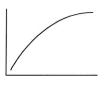
maturity
Diagram 7: Positive yield curve
- Negative, or inverse: this is the opposite of the positive yield curve. An inverse yield curve reflects a situation where short-term interest rates are higher than long-term rates. This may indicate that there are expectations of falling interest rates in the future. A negative yield curve is consistent with expectations of falling inflation (or disinflation) over the longer term. It could also be a reflection of government monetary policy attempting to reduce interest rates in a sluggish economy. In such a case, investors may choose to lengthen the maturity of their debt portfolios and even purchase more bonds if they expect inflation to fall in the future.
yield
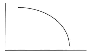
maturity
Diagram 8: Negative yield curve
- Flat: a flat yield curve reflects market expectations that interest rates will remain stable in the future. It may also indicate a transitional stage from a positive to an inverse yield curve, or vice versa.
yield
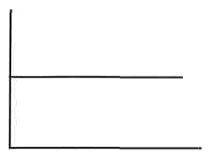
maturity
Diagram 9: Flat yield curve
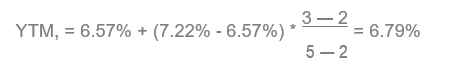
Ideally, we should plot the yield curve by using bonds with different maturities issued by the same issuer. If there is no example of a bond at a particular maturity, the YTM on the missing bond for that maturity can be interpolated from the nearest lower maturity and the nearest higher maturity, using the following formula:
YTM = YTML + (YTMH – YTML) x (N-L) / (H-L)
where N = the term to maturity for which we want to compute the YTM; H = the nearest higher term to maturity; and
L = the nearest lower term to maturity
Suppose that we have only the yields to maturity on a two-year bond and a five-year bond, which are 6.57% and 7.22% respectively. The YTM of a three-year bond should be:
Implied forward rates
With the spot-rate yield curve, we can determine implied forward rates. A forward rate is the rate of return on a transaction that will take place in the future although all the contract terms are set out in the present. For example, consider a one-year zero-coupon bond and a two-year zero coupon bond. The spot rates (the same as the yields to maturity for zero-coupon bonds) for the one-year and two-year bonds are r1 and r2 respectively. If we sell $1 of the one-year bond short, we expect to have a cash inflow of $1 now and a cash outflow of $(1 + r1) in a year’s time. Simultaneously, if we buy $1 of the two-year bond now, we expect to pay a cash flow of $1 now and to receive a cash inflow of $(1 + r2)2 in two years’ time. The combined strategy of selling $1 of the one-year bond and buying $1 of the two-year bond will have a zero net cash flow now, a cash outflow of $(1 + r ) in a year’s time and a cash inflow of $(1 + r2)2 in two years’ time. This is similar to a forward contract, and its rate of return is called the implied forward rate (f2), which can be determined with certainty because we derive the one- and two-year spot rates directly from the yield curve. The formula for the implied forward rate is:
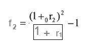
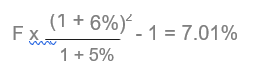
For example, the implied forward rate should be 7.01%, if the spot rates of one- and two-year bonds of the same credit risk class are 5% and 6% respectively:
1.2.2 Interest rate theories
As discussed, both the spot rates (observed from the yield curve) and the implied forward rates are certain, so we are mostly interested in estimating the expected future spot rates. The question here is whether we can use the certain implied forward rates to estimate uncertain expected spot rates. The answer to this question will also tell us about the likely shape of the yield curve. There are three interest rate theories that attempt to provide an answer to this question: the unbiased expectations hypothesis, the liquidity preference theory and the market segmentation theory. Before we discuss these hypotheses, let us consider two alternative investment strategies. The first is to invest in a two-year zero-coupon bond with a spot rate of r , while the second is to invest in a one-year zero-coupon bond with a spot rate of in and roll it over to another one-year bond in a year’s time with an expected spot rate of E(l 2) Both strategies involve an investment horizon of two years. At the end of the investment horizon, the cash inflow for the first strategy is (1 + r )2 and for the second (1 + r )[1 + E( r2)]
Unbiased expectations hypothesis
The unbiased expectations hypothesis states that the first strategy (long-term bonds) and the second (short-term bonds) are equivalent and that they provide the same return. Hence, the implied forward rate is an unbiased estimator of the expected spot rate. In other words, the shape of the yield curve results from the market participants’ interest rate expectations. If we expect the interest rate to rise, the yield curve is upward sloping. If we expect it to fall, the curve is downward sloping. If we expect the interest rate to be constant, the curve is flat. If we expect the medium-term interest rate to rise, but the long-term interest rate to fall, the curve is humped. This hypothesis attempts to explain why the yield curve takes a particular shape. Under the hypothesis, the observation that the curve is generally upward sloping can only be explained by the assumption that we expect the interest rate to rise more often than fall, e.g. because of inflation expectations.
Liquidity preference theory
The liquidity preference theory states that investors prefer the second rolling-over strategy (short-term bonds) to the first (long-term bonds), which involves a bond with longer maturity and hence lower liquidity. Investors need a higher required rate of return to compensate for liquidity risk. This type of risk premium is called the liquidity or term premium. Under this theory, the expected spot rate is equal to the implied forward rate minus the liquidity premium, which can be estimated using past data. The upward bias on the longer-term bonds generally means that the yield curve is upward sloping. However, it cannot explain other yield curve shapes.
Market segmentation theory
The market segmentation theory, also known as the preferred habitat theory, states that the markets for short-term bonds and long-term bonds are separate and independent of each other, because bond sectors are segmented by institutional investors with different needs. A bond sector’s interest rate is determined by the demand and supply conditions in that sector alone. In other words, there is no relationship between the first strategy (long-term bonds) and the second (short-term bonds). Under this theory, the yield curve can take any shape, and the theory is the one most favoured by practitioners.
All three theories have their own merits. They each illustrate the factors that we need to consider when predicting future interest rates – inflation expectations, liquidity preference and the demand and supply conditions in a particular bond sector.
1.3 Bond valuation
- Valuation of bond by yield to maturity
The price or value of a coupon bond is the sum of the present values of all future cash flows (i.e. assuming that the bond is held to maturity, the sum of the present values of all interest payments and the principal repayment amount). For example, if a 3-year coupon bond pays its coupon semi-annually, there is one coupon payment every half-year and a total of six during the life of the bond, i.e. at years 0.5, 1.0, 1.5, 2.0, 2.5 and 3.0 respectively. The principal of the bond will be repaid at maturity, i.e. at year 3.0, together with the final coupon payment.
The cash flows involved in the above coupon bonds are illustrated below:
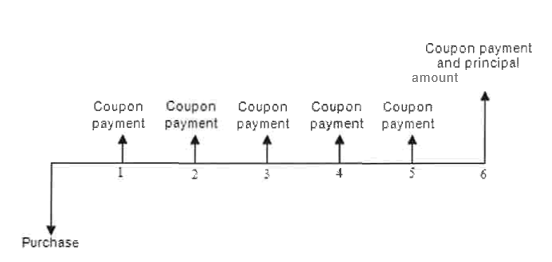
Note: This diagram assumes semi-annual coupon payments, 6 payments over 3 years.
Diagram 10: Cash flows involved in coupon securities
To calculate the price of this coupon bond, the payment received in each period, i.e. every 0.5 years, has to be discounted to the present time. The sum of these individual present values is the fair price of the bond.
Mathematically, this is expressed as follows:
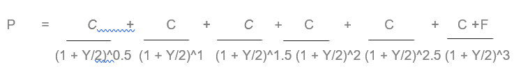
where:
P fair price
C coupon
F face value
y yield per annum
The coupon of a bond is usually quoted as a percentage of its face value. For example, if a coupon bond with a face value of $1,000 pays a coupon of 5% annually, a coupon of $50 (or $1,000 x 5%) is paid every year. However, if the coupon is paid half-yearly, a coupon of $25 (or $1,000 X 5% / 2) is paid every six months.
A 2-year bond has a face value of HKDl,000 and a yield of 10%. A coupon of HKD100 is paid annually. What is the bond price?
P = 100 / (1 + 10%)’ + 1,100 / (1 + 10%)2 = 1,000
A 2-year bond has a face value of HKD1,000 and a yield of 10%. A coupon of HKD80 is paid annually. What is the bond price?
P = 80 / (1 + 10%)’ + 1,080 / (1 + 10%)2 = 965.29
A 2-year bond has a face value of HKD1,000 and a yield of 10%. A coupon of HKD120 is paid
annually. What is the bond price?
P = 120 / (1 + 10%)’ + 1,120 / (1 + 10%)2 = 1,034.71
For the price of a zero-coupon bond, the following formula applies:
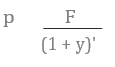
where:
P price
F face value
y discount rate
t time to maturity
A 2-year zero coupon bond has a face value of HKD1,000 and a yield of 10%. What is the bond price?
P = 1,000 / (1 + 10%)2 = 826.44
For the price of a perpetual bond, the following
formula applies: P = C / Y
A perpetual bond with a face value of HKD1,000 has a coupon rate of 8% and a yield of 10%. What is the bond price?
P = 1,000 • (8% / 10%) = 800
1.3.2 Valuation of bond by spot rates
As mentioned in section 3.5.1, the simplest way to calculate the value of a bond is to take the cash flows of the bond till its maturity and then discount them by means of a single discount rate. The method is quick but not very accurate because we have always assumed that the interest rate is constant over time. However, one major factor that influences the spot rate is the bond maturity. Hence, the one-year interest rate is different from the two-year rate. However, even if two bonds have the same maturity, they can still have different spot rates because of their different credit risk. In practice, we can determine the spot rates for bonds through observable bond prices in the same credit risk class (the same credit rating). The simplest case is when we consider a series of zero-coupon bonds with different maturities. The YTM of a zero-coupon bond with a particular maturity is the spot rate at that maturity.
Suppose we want to calculate the value of a $1,000 par, 5% coupon, 4-year maturity bond. We also have the following spot rates for the next four years:
| Period | Spot Rate |
| l | 4.00% |
| 2 | 4.35% |
| 3 | 4.60% |
| 4 | 4.70% |
Assuming it is an annual pay bond, the bond will have the following cash flows.
Year l: $50
Year 2: $50
Year 3: $50
Year 4: $50 + $1,000
The value of the bond can be calculated by discounting these cash flows by their respective spot rates.
bond value = 50/(1.04) + 50/(1.0435)2 + 50/(1.046) 3 + 1,050/(1.047) = $1,011.465
1.3.3 Benchmark yield curve
The benchmark yield curve is used to price private debt securities and assist in maintaining an active and liquid debt market. Government securities are assumed to be risk-free (if they are highly rated) and are often called benchmark issues. The risk-free yield curve, serving as the benchmark yield curve, refers to the risk-free spot rates which are calculated using the stripping or bootstrapping technique based on benchmark securities.
In the US, the benchmark yield curve is derived from treasury bills, notes and bonds. In Hong Kong, the curve is derived from EFBs and EFNs.
1.3.4 Yield spread
A yield spread is measured by the difference between the yields on two bonds. The first is the one under consideration, while the second is the reference bond. The difference is usually measured in basis points. The spread between the interest rates in two bond sectors with the same maturity is called an inter-market sector spread. The spread between two issues within a bond sector is referred to as an intra-market spread. If the reference bond is a government security assumed to be risk-free, the spread is known as the credit spread, which is a measure of the credit risk premium of the bond under consideration. It reflects the bond’s credit risk and can be used to price a newly issued bond with the same credit risk. Yield spreads can be measured on an absolute basis (called the absolute yield spread), on a relative basis (called the relative yield spread) or as a ratio (called the yield ratio) as follows:
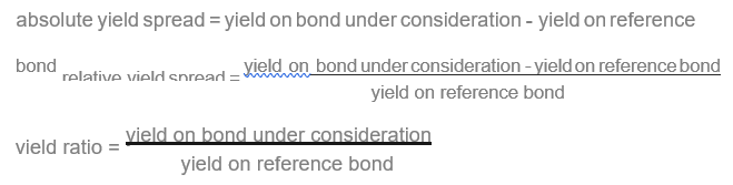
Suppose that the yields to maturity of a three-year $1,000 par 5% bond and a three-year government bond are 5.25% and 5% respectively. Compute the absolute yield spread, the relative yield spread and the yield ratio of the two bonds.
absolute yield spread = 5.25% — 5% = 0.25%
relative yield spread = (5.25% — 5%) / 5% = 5%
yield ratio = 5.25% / 5% = 1.05
CRAs usually provide the credit spread information and the default probability. A typical example of a credit spread is given below.
Table 2: Credit spread and default probability
| Synthetic rating | Credit spread | Default probability |
| AAA | 0.91% | 0.01% |
| AA | 1.43% | 0.28% |
| A | 1.95% | 0.53% |
| BBB | 2.98% | 2.30% |
| BB | 5.40% | 12.20% |
| B | 8.24% | 26.36% |
| CCC | 19.99% | 46.61% |
The credit spread shows the risk premium of a bond with a certain credit rating. It also helps to price a newly issued bond at that credit rating.
In practice, pricing of a bond can be represented as follows:
= absolute yield (e.g. 3%) represented by the credit curve of the bond issuer at a particular maturity, or
= spread to treasury (90bps) = US treasury (2.1%) + UST spread (90bps) (the difference between the issuer’s credit curve and the treasury curve) at a particular maturity, or
= spread to swap (50bps) = USD LIBOR (2.5%) + USD LIBOR spread (50bps) (the difference between the issuer’s credit curve and the swap curve) at a particular maturity.
Short-term drivers of interest rates
Monetary policy of central banks
A central bank can make use of open market operations, discount rates and reserve requirements to affect the short-term interest rate.
Open market operations can be used for expansionary or contractionary monetary policies. In the former case, the central bank purchases securities from the banks and injects money into the banking system. Hence the money supply increases and the interest rate decreases. On the other hand, with a contractionary monetary policy, the central bank sells securities to the banks and withdraws money from the banking system. Hence the money supply decreases and the interest rate increases.
In most countries, central banks are always the lenders of last resort and charge interest on short-term lending to banks. A lower discount rate encourages banks to borrow from the central bank. Hence the money supply increases and the interest rate decreases.
In addition, central banks can adjust the bank reserve requirement to influence the interest rate. A lower reserve requirement allows banks to increase their lending. Hence the money supply increases and the interest rate decreases. On the other hand, a higher reserve requirement causes banks to decrease their lending. Hence the money supply decreases and the interest rate increases.
Inflationary expectations
Price stability or an appropriate inflation rate is always the policy target of central banks in most countries. When there is an expectation of inflation leading to the expected rate of inflation exceeding a central bank’s targeted inflation rate, the central bank can increase the short-term interest rate to curb inflation. The higher short-term interest rates will rise, via the financial markets, and the cost of funds will in turn reduce consumer demand and investments, lessening inflationary pressures.
Globalization and exchange rates
The increasing connection of trade and financial transactions leads to more frequent and larger capital flows among countries. An inflow of capital into the debt market of a particular country, the result perhaps of its booming economy and stable sovereign credit rating, can increase the demand for sovereign and corporate bonds in that country, and hence drive down the interest rate.
In addition, the inflow of capital would also affect the exchange rate, as the higher demand for the local currency would lead to a stronger exchange rate, potentially leading to a decline in its exports and an increase in its imports. A weaker economic performance due to the drop in net exports and the potential deflationary effect would lead the central bank to lower the interest rate.
Long-term drivers of interest rates
Short-term interest rates and inflationary expectations
In general, short- and long-term interest rates tend to move in the same direction. For instance, a higher short-term interest rate would re-direct capital to move from the bond market to the money market, causing the bond price to decline and hence the interest rate to increase.
Also, long-term interest rates will normally be higher than short-term rates because of inflationary expectations.
Fiscal policy of governments
In an expansionary fiscal policy, the government may lower the tax rate and increase public spending to stimulate the economy. When the government encounters a fiscal deficit and hence needs to issue new government debt to support its expansionary fiscal policy, there will be a greater supply of bonds in the market. Bond prices may fall and yields/interest rates increase.
On the other hand, with a contractionary fiscal policy, the government may increase the tax rate and reduce public spending to slow down the over-heating economy. When the government attains a fiscal surplus and does not need to issue any new government debt, there will be fewer bonds in the market, prices may increase and yields/interest rates fall.
Competition in financial markets
When there are many banks in the loan market and the fund managers in the capital market, debt borrowers, especially those with a higher credit rating, can leverage this ample supply of liquidity to lower their debt funding costs on their loan and bond refinancing. This is especially true in markets like Hong Kong, where many international, regional and local banks are competing for loan business in a limited pool of high quality corporate borrowers.
Price/yield levels of other asset classes
Equity and bonds are the two main asset classes in the global investment community. In the past few years, the equity market has not been performing well, and has therefore encouraged a large quantity of capital to switch to the bond market for better investment opportunities, especially in the high yield sector. The increased demand for bonds has led to over-subscription of many new bond issues, especially in Asia, and this has been driving down the interest rate in the bond market. Sovereign and corporate bond issuers have been leveraging this situation to lower their bond coupons on refinancing or exercising their call options on bonds. Therefore, long-term interest rates will reflect the preferences and expectations of investors in the various asset classes.
It should be noted that the above discussion of various drivers/factors is a simplified version only. In reality, the determination of interest rates is a highly complex matter, with interactions among various factors and market forces.
Risks associated with bond investment
While credit or default risk is the major risk of investing in bonds, investors should also be aware that there are other risks associated with fixed income investment.
Credit risk
Default risk
Default risk is the credit risk that the bond issuer will not pay the interest and/or the principal 1) in full and 2) on time according to the terms and conditions of the bond prospectus. Bond credit ratings primarily offer a view on the credit/default risk of investing in bonds.
High yield bonds are often rated below investment grade or unrated. While ratings from the CRAs do not guarantee the creditworthiness of the issuers, investing in non-investment grade or unrated bonds may incur a higher risk of default by the issuers. Also, high yield bonds are more vulnerable to economic changes. During economic downturns, the value of these bonds typically falls more than that of investment graded bonds because investors become more risk-averse and default risk rises.
A higher credit rating denotes a lower default probability (the likelihood of default according to S&P and Fitch) or lower expected loss (reflecting both the likelihood of default and the loss given default according to Moody’s), and vice versa.
Bonds occasionally carry split ratings i.e. different ratings assigned to the same entities by the rating agencies. It is more prudent to look at the lower ratings by one of the two or even three rating agencies in monitoring the credit performance of the bond portfolio.
Credit spread risk
The credit spread of a bond primarily reflects the credit risk of a bond issuer relative to that of the risk-free issuer. If such relative risk is expected to be higher, then the bond credit spread will be widened and this will result in a lower bond price.
Downgrade risk
If a bond issuer’s financial condition deteriorates and is no longer up to the initial rating assigned, its credit rating will either be put on negative rating watch or negative rating outlook (which indicate a higher likelihood of rating downgrade in the future), or be downgraded immediately. In either of these cases, the bond price will fall to reflect such downgrading.
As CRAs have been criticized for massive and sudden downgrades of structured bonds and sovereigns without any prior warning to the market, nowadays all bonds which are likely to be downgraded will go through the negative rating outlook and/or negative rating watch stages, before eventually being downgraded. Bond prices should have reacted to the announcement of negative rating outlook/watch, rather than the actual downgrade. Private wealth managers should closely monitor such announcements of downgrade risk.
CRAs tend to cap the ratings of corporates and banks at their government ratings. Most bank ratings will in fact be downgraded once their government ratings are downgraded, as we have seen many times in Europe. Hence a more effective approach for private wealth managers to monitor the downgrade risk of their customers’ bond portfolios is monitoring the CRA actions on the sovereign ratings.
Market risk and interest rate risk
A bond price is equal to the sum of the present value of future bond coupons and principal. If an investor needs to sell a bond prior to maturity, an increase in the interest rate would lead to a fall in the present value of future cash flow streams and hence the investor will suffer from a capital loss. This is the market or interest rate risk of investing in bonds.
Since bonds are mainly traded over the counter, and data providers like Bloomberg and Reuters can only provide indicative bond pricing (rather than a firm bid/ask), private wealth managers and investors should approach the banks which are more active dealers in particular bonds (e.g. US investment banks for USD denominated bonds or Chinese investment banks for dim sum bonds) to obtain more relevant bond pricing to facilitate the monitoring of their bond portfolio market risk.
Measures of interest rate risk
Duration is a measure of the responsiveness or sensitivity of the bond price with respect to changes in market interest rate.
Macaulay duration represents the weighted average maturity of a bond, i.e. weighted average term-to-maturity of a security’s cash flows, which is a measure of the effective maturity of a bond. The present value of each cash flow is weighted by the period when it is due, and the resulting sum is divided by the market price. Macaulay duration is a time measure, with years as units, and measures the percentage change in bond prices with respect to a percentage change in the interest rate.
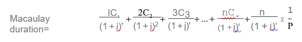
where C = coupon;
i = yield;
M = maturity value; and
n = number of coupon payments per yr
P = current price of the bond.
Modified duration measures the percentage change of price with respect to yield. modified duration = Macaulay duration / (1 i/n),
where i = yield; and
n = number of coupon payments per year.
Example
A 3-year USD100 million bond with a 6% coupon yielding 4%. The Macaulay duration is calculated in the following steps:
- Present values of each of the individual cash flows are calculated by discounting the market interest rate of 4%. The sum of these present values is the market value (price) of 105.55.
- Each of the present values is time-weighted by multiplying them by the period until the cash flow receipt e.g. 94.23% x 3 = 2.827. These items are summed and divided by the market value to obtain the Macaulay duration i.e. 2.9956/1.0555 = 2.838 years. The following table gives the details.
| Year (T) | Cash Flow (CF) | Present Value (PV) of CF | T • PV of CF |
| 6 | 5.77 | 5.77 | |
| 2 | 6 | 5.55 | 11.09 |
| 3 | 106 | 94.23 | 282.70 |
| 105.55 | 299.56 |
modified duration = Macaulay duration/(1 + i/n) = 2.838/(1 + (0.04/1)) = 2.729
If the interest rate subsequently increases by 0.10%, the bond value is expected to change as follows:
% price change = -modified duration x yield change = -2.729 x 0.10%= -0.27% price change = 105.55 x -0.27% = -0.2850
bond value = 105.55 – 0.2850 — 105.265
A 0.10% increase in the interest rate leads to a 0.27% decrease in bond value.
Duration is a linear approximation of the price-yield relationship. Therefore, it only applies when there is a small change in interest rates. To capture the curvature of the price-yield relationship, we need a measure of convexity to show the rate of change in modified duration as the yield changes. The more convex a bond is, the more its duration will change with interest rate change.
Convexity is measured in years and generally increases with maturity and decreases with increasing coupon rate and yield. Technically, this is obtained from the second derivative of the price-yield curve.
Re-investment risk
Reinvestment risk is the risk of the falling interest rate at which interim cash flows can be reinvested. Reinvestment risk is often associated with high bond coupons as well as bond prepayment.
In addition, it is closely related to the callable bond when the issuer redeems the bond early in order to take advantage of the falling interest rate and lock in a lower coupon. Other things being equal, a zero coupon bond usually has less reinvestment risk than a coupon bond because the entire cash flow is paid only at maturity.
There are three factors which affect the call risk, as follows:
- the cash flows become uncertain because of the call provision or prepayment right;
- the risk of reinvesting the cash flows at a lower yield (the reinvestment risk); and
- the potential for price appreciation is reduced because of a cap on the bond price (call price or the principal), i.e. price compression.
It should be noted, however, that in bond investment the interest rate risk (causing bond prices to drop in an increasing interest rate environment) will offset the reinvestment risk (allowing bondholders to reinvest at a higher coupon bond in an increasing interest rate environment).
Inflation risk
Inflation lowers the purchasing power. If the inflation rate is higher than the coupon rate, the real value of the future bond coupons and principal will decline, and the purchasing power of such future cash flow streams will be lower.
Even if the inflation rate is lower than the coupon rate, a rising inflation rate will gradually erode the purchasing power of the future bond coupons and principal.
Liquidity risk
Liquidity risk refers to the discount from the par value when a bond is quickly sold in the market before the maturity. There are many different measures of bond liquidity, but the most common on is the bid-ask spread quoted by dealers. In general, the wider the dealer spread, the higher the liquidity risk.
Bonds are generally less liquid than stock. As a result, even if a bond is not subject to any imminent default, bond investors still need to suffer a loss in selling such a bond prior to maturity. Structured bonds like ABS and CDO are less liquid than plain vanilla bonds.
Liquidity risk is very important in Asia, where most bond investors are buy-and-hold investors. Hence private wealth managers should advise their customers to hold a more diversified bond portfolio, rather than a portfolio of the same size comprising one or two bonds, in order to speed up the sale and minimize the discount on a bond sale if it becomes necessary.
Currency risk
Currency or exchange rate risk refers to a change in one currency against the other which causes bond investors to suffer from losses. This can be looked at from two perspectives.
First, if an investor is managing a USD fixed income portfolio but invests in non-US dollar, e.g. Singapore dollar (SGD), bonds without entering into any currency hedge, then a depreciation of Singapore dollar against US dollar through the bond tenor would result in a lower USD equivalent of the SGD coupons and SGD principal to be received.
Second, if a Malaysian company, for instance, issues USD bonds without entering into any currency hedge, then a depreciation of Malaysian ringgit (MYR) against US dollar means the issuer needs to put in more Malaysian ringgit to repay the same amount of USD coupons and USD principal. While
this will not directly affect the currency exposure of a bond investor, such currency move would increase the credit risk of the issuer and hence affect the investor.
Event risk
In recent years, the managements of many corporations have tried to boost their shareholder value by undertaking leveraged buyouts, restructurings, mergers and recapitalizations. Such corporate activities are usually highly leveraged to take advantage of the current low interest rate environment for debt funding.
In practice, event risk is far more difficult to predict and monitor, especially for bond issuers not listed in any stock market. Private wealth managers and investors are therefore advised to focus more on issuers listed in the stock market as there is far more public information (e.g. annual and interim reports, equity research analyst reports, etc.) to monitor their corporate activities.
Leverage risk
Most private wealth institutions these days offer leverage to their customers for bond investments. Leverage depends on the bond rating – moderate for high yield bonds but high for investment grade bonds. Leverage also depends on the liquidity of the bonds.
Since most bonds are still traded on the over-the-counter market, prices and liquidity are not transparent and prices can be volatile, especially during a panic situation. Hence customers of private wealth institutions need to be aware of all the risks of investing in bonds, in particular the credit risk and market (interest rate) risk, which would have immediate impact on the bond pricing and potentially lead to margin calls.
It should be noted that leverage risk does not just apply to bonds but also to other asset classes.
A case study in risk analysis for customer’s bond portfolios
If a customer of a private wealth institution has the following bond portfolio (as of August 2014) and asks for your help in commenting on the portfolio risks, what can you say?
Table 3: Bond portfolio
| Bonds | Coupon (%) | Moody’s rating | S&P rating | Maturity | Currency | Purchase price | YTM (%) | YTC (%) |
| China property developer | 8.875 | Ba2 | BB- | 28/04/2017 | USD | 104.58 | 6.99 | 5.37 |
| China mining company | 5.73 | Bal | BB+ | 16/05/2022 | USD | 94.08 | 6.72 | 6.72 |
| Russia bank | 6.875 | Baa2 | BBB- | 29/05/2018 | USD | 100.64 | 6.68 | 6.68 |
| US Gaming Company | 7.75 | B3 | B+ | 15/03/2022 | USD | 115.45 | 5.26 | 5.26 |
| French bank perpetual | 8.25 | BB+ | BB- | N/A | USD | 106.61 | 7.68 | 6.465 |
The bond portfolio concentrates on non-investment grade bonds, which are subject to a higher default risk.
All five bonds have split ratings, i.e. different ratings assigned to the same entities by the CRAs. It is more prudent to look at the lower ratings by one of the two CRAs in monitoring the credit performance of the bond portfolio.
The portfolio also concentrates on bonds with long maturities, including perpetual bonds. It will be _. subject to a higher market risk when the interest rate increases in the future. Even the rumour of an
interest rate hike could easily cause bond prices to fall. Most private wealth institutions will advise their customers to restrict the bond portfolio duration to not more than five years, or an even shorter period.
Given political developments in Russia and Ukraine, Russia would be subject to a potential sovereign rating downgrade and hence put downgrade rating pressure on all the Russian banks and corporates, including the Russian bank in the portfolio.
YTC rather than YTM should be considered in reviewing the yield performance of the portfolio.
2. Bond management strategies
2.1 Active management strategies
Active management strategies involve taking active bond positions with the objective of obtaining a return higher than the benchmark rates such as bond indices.
Credit strategies
Quality swap
A quality swap is the active bond management strategy of moving from one quality group to another, with investors’ expectations of a change in the economic conditions of a country.
If the investor expects an economic recession, he will long high quality bonds and short low quality bonds (or change the bond fund allocation by selling some of the low quality bonds and buying more high quality bonds).
Once the expected recession materializes, the lower quality companies will suffer from declining profits and cash flow and their bond prices will drop. At the same time, higher quality companies will still survive and their bond prices will not change significantly (they may even increase when the flight to quality among bond investors occurs during a recession). Investor will therefore profit from both the high quality bond (long) and low quality bond (short) positions.
If the investor expects an economic expansion, he will short the high quality bonds and long the low quality bonds (or change the bond fund allocation by selling some of the high quality bonds and buying more low quality bonds).
Once the expected expansion materializes, both high and low quality companies benefit. But the spread between high and low quality bonds will narrow during an economic expansion and hence the investor will profit from both the high quality bond (short) and low quality bond (long) positions.
Credit analysis strategy
A credit analysis strategy involves a fundamental credit analysis of corporate or sovereign bonds in order to identify potential changes in default risk. The information is then used to identify bonds to include or exclude in a portfolio or investment strategy.
If bond rating changes can be projected prior to any rating action announcement, bond investors can realize gains by buying bonds likely to be upgraded, and avoid losses by selling or not buying bonds they expect to be downgraded.
Credit analysis can be effected through basic fundamental analysis of the bond issuer: qualitative and quantitative analysis.
Qualitative analysis, which typically has more weight for investment grade bond issuers, involves the following analysis:
- Industry risk: the focus is on the cyclicality/volatility of an industry sector.
- Operating environment: the focus is on the impact of social and demographic changes on a country and/or its industry sector.
- Market position: a dominant market position or share can increase a company’s ability to influence both its own and the market’s pricing.
- Management quality: the focus is on whether a company management has met its past projections or promises.
- Corporate governance: a company management with good corporate governance always considers the interest of various stakeholders (including the bondholders) in its decision-making.
- Legal and regulatory issues: a country or industry with a sound legal system and tight regulation will benefit a company over the long term.
Quantitative analysis, which typically has more weight for non-investment grade bond issuers, involves the following:
- Earnings and cash flow: a measure of the company’s ability to generate internal operating cash flow for debt service, as well as ongoing investment needs.
- Capital structure: the mix of debt and equity demonstrates management’s attitude to risk.
- Financial flexibility: a measure of the company’s ability to cope with periodic volatility, caused by unexpected events.
- Coverage ratio: a measure of the company’s cash generating ability relative to its finance costs,
e.g. interest coverage ratio.
- Leverage ratio: a measure of the company’s debt burden relative to its cash generating ability,
e.g. debt ratio and debt-to-equity ratio.
- Profitability ratio: a measure of the company’s profitability from one period to the next on a like-for-like basis, e.g. gross profit margin, net profit margin, return on assets and return on equity.
Interest rate anticipation strategies
Riding the yield curve
When the yield curve slopes upward, bond investors will ride the curve to increase their bond investment returns by buying bonds with maturities longer than the desired holding periods, and selling them to profit from falling bond yields as maturities decrease with the passage of time
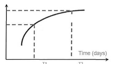
Diagram 11: Positive yield curve strategy
Interest rate timing
Bond management strategy based on changes in the expected interest rate level is very simple.
- If interest rates go down, buy bonds with the longest possible duration.
- If interest rates go up, sell bonds to shorten the bond portfolio duration.
Passive management strategies
Buy-and-hold strategy
In the buy-and-hold strategy, a portfolio manager chooses a portfolio of bonds, bearing in mind the objectives of and constraints on the investor, and holds this portfolio to maturity. He will choose bonds with the desired qualities such as coupon levels, credit risk, maturities and indenture provisions. The bonds’ maturities will be close to the investor’s investment horizon to reduce price and reinvestment risk. This does not mean that the portfolio manager will not choose bonds with attractive maturity and yield features. In fact, the manager has to use his knowledge of the markets and bond issues to look for attractive yields.
Indexing
Indexing is used to form a portfolio that mimics the composition of a specified bond index. The portfolio manager’s performance is evaluated by examining the tracking error between the portfolio return and the bond index return. The size of the portfolio return will depend on how familiar the manager is with the various characteristics of the bond indices and how these change over time.
Full replication of a bond index is impractical, as it involves too many bonds. Generally, stratified sampling is used to choose a representative subset of the bonds in the index. This strikes a balance between transaction costs and the tracking error, which is the difference between the bond portfolio return and the index return.
Whether the investor adopts an active or passive bond management strategy, the investors need to consider the weighting of bonds and other asset classes in constructing their bond portfolios:
- Low risk: the investor can allocate between 30% and 40% of his funds to bonds. Within the bond portfolio, 80% can be allocated to developed markets and 20% to emerging markets.
- Medium risk: the investor can allocate between 20% and 30% of his funds to bonds. Within the bond portfolio, 80% can be allocated to developed markets and 20% to emerging markets.
- High risk: the investor can allocate not more than 10% of his funds to bonds. Within the bond portfolio, the majority can be allocated to the emerging markets.
Again, the above only serves as a rough guide, and consideration should normally be on a case-by-case basis. Apart from the notion of developed versus emerging markets, consideration should also be given to other relevant factors, such as credit rating, term-to-maturity, seniority and any special features or terms of the bond that may render it unsuitable for certain customers’ circumstances.